A primer on finite element methods
Contents
A primer on finite element methods#
Galerkin’s method: A recipe to discretize partial differential equations#
The general recipe#
Galerkin’s method is an general approach to solve partial differential equation numerically by transforming them into a system of discrete equations. The computed solution to the discrete equations can then be thought of as an approximation to the solution of the original PDE. Figure Fig. 1 summarizes the four stages of the discretization approach which we describe next. As usual, we will use the Poisson problem as a guiding prototype example.
Note
The following recipe is deliberately kept vague. Details such as boundary conditions, suitable function spaces, and
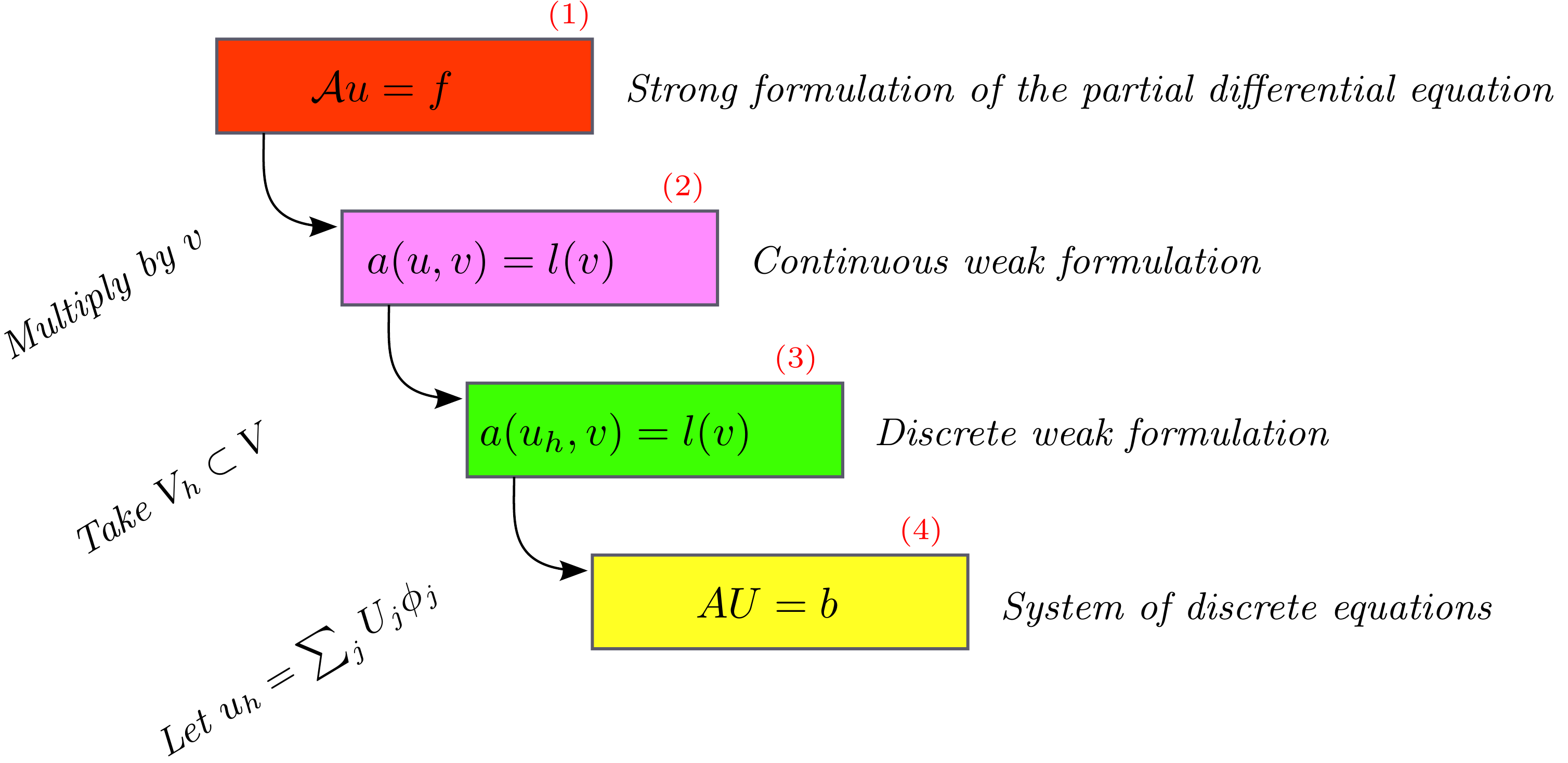
Fig. 1 The four stages of Galerkin’s method to discretize partial differential equations.#
- Stage 1
Strong formulation of the PDE
Starting point is a partial differential equation
in strong form: for given function \(f:\Omega \subset \RR^n \to \RR\) and partial differential operator \(\mcA\), we assume that the function \(u: \Omega \to \RR\) satisfies the relation (22) pointwise so that \(\mcA u(x) = f(x)\: \forall x \in \Omega\).
Our favorite example is of course the Poisson problem with homogeneous Dirichlet boundary condition:
- Stage 2
Continuous weak formulation of the PDE
Find \(u \in V\) such that
The standard approach to obtain a weak formulation is to multiply with the strong form of the PDE with appropriate test functions which satisfy appropriate smoothness assumptions and —if required— boundary conditions.
For the Poisson problem with homogeneous Dirichlet b.c. we saw previously that we arrived at the weak formulation: Find \(u \in V := H^1_0(\Omega)\) s.t. \(\forall v \in V\)
- Stage 3
Discrete weak formulation of the PDE
By choosing a suitable approximation space \(V_h \subset V\) with finite dimension \(N = \dim V_h\), we obtain the discrete weak formulation:
Find \(u_h \in V_h\) such that
- Stage 4
Formulation as system of discrete equations
To translate the now finite-dimensional problem (25) into a discrete system of equations, we choose a basis for the discrete function space
First observe that the problem (25) is then equivalent to seek a \(u_h \in V_h\) such that
since \(a(\cdot, \cdot)\) and \(l(\cdot)\) are linear in their respectively second and first slot.
The second step is now to rewrite \(u_h = \sum_{j=1}^N U_j \phi_j\) with the help of the basis functions and to insert this representation into (26) to obtain a discrete system of equations for the coefficient vector \((U_i)_i^N \in \RR^N\). If \(a(\cdot,\cdot)\) is not linear in the first slot —think of nonlinear PDEs such as the Navier-Stokes equations—, then the resulting system is truly nonlinear. But for weak formulation one linear PDEs, the linearity in the first slot of \(a(\cdot, \cdot)\) allows us to to cast (26) into a linear system
with \(A \in \RR^{N\times N}\) and \(b \in \RR^N\) since
Abstract error theory#
Lemma 3 (Galerkin orthogonality)
Assume that \(V_h \subset V\) and that \(u \in V\) and \(u_h \in V_h\) solve the continuous weak formulation (24) and the discrete weak formulation (25), respectively. Then the error \(u-u_h\) satisfies the orthogonality relation
Proof. If \(v_h \in V_h \subset V\), then the continuous \(u\) and the discrete solution \(u_h\) satisfy
Subtracting the second equality from the first yields (29).
Lemma 4 (Cea’s lemma)
Assume that
\(V_h \subset V\)
the continuous weak formulation (24) satisfies the assumptions of the Lax-Milgram theorem.
\(u \in V\) is solution to the continuous weak formulation (24)
\(u_h \in V_h\) is solution to the discrete weak formulation (25)
Then \(u_h\) satisfies a quasi best approximation property in the sense that
holds for the error \(u-u_h\). Here \(C_a\) and \(\alpha\) are the boundedness and ellipticity constants for \(a(\cdot, \cdot)\) appearing the assumptions for the Lax-Milgram theorem.
Proof. Let \(v_h \in V_h\) be fixed but arbitrary, then we wish to show that
The proof of this inequality is rather short. Its main essence consists of three estimates where we first use coercivity of \(a(\cdot, \cdot)\) to relate \(\|u-u_h\|\) to \(a(\cdot, \cdot)\), then add and substract the given \(v_h\) and apply Galerkin orthogonality, and finally boundedness of \(a(\cdot, \cdot)\) is exploited to estimate the resulting expression. To this end, we see that
Assuming that \(\| u - u_h \| \neq 0\) (otherwise (31) is trivially satisfied), we can divide (32) by \(\| u - u_h \|\) and \(\alpha\) to see that