Dimensional Splitting with Grid Refinement
Local Grid Refinement
|
The underlying grid in the dimensional splitting algorithm is some sense an
artifact introduced to simpify the process of determining the initial data for
the next fractional step. After each front tracking pass, the solution is
represented on a finer, but nonuniform grid. When projecting the solution some
finescale information is lost. In fact, experience has shown that for CFL
numbers slightly above unity, the projection operator is contributing most to
the numerical error of the method. By introducing local grid
refinement we can hope to improve the projection operator.
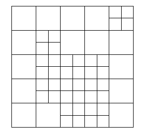
We introduce grid refinement by local partition of grid blocks as
indicated in Figure 1. This partition may be fixed, or
vary throughout the computation. This obviously leads to a reformulation of
the front tracking algorithm, since we have rows (or columns) in the
grid containing refined blocks. Inside each tube (a section of a row/column
consisting of cells of the same type, coarse or refined) the front tracking
algorithm works as before, but on the interface between coarse and refined
cells we must do something new.
|

Figure 1: Local partition of grid blocks.
|
Modified Front Tracking Algorithm
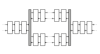
Inside each tube the data structure introduced earlier can be utilised. To
couple coarse and refined tubes, we introduce a special (static) front, as we
did for the boundary. The front points to its nearest neighbour in the coarse
tube and to the nearest neighbour in each refined tube. This is illustrated
in Figure 2.

Figure 2: Example of a front list. The static fronts are shaded.
|
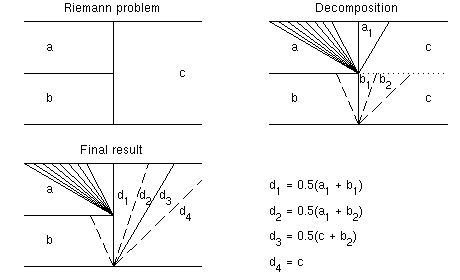
At an interface, the Riemann problem is two-dimensional. However, the flux
function is nonzero only along the tube. Therefore the Riemann problem is
simply a series of one-dimensional Riemann problems, one for each refined
tube. Each Riemann problem will in general give waves that propagate in both
directions, into the refined tube and into the adjacent coarse tube. The
fronts propagating into the refined tube can simply be inserted into the
corresponding front list. The fronts that propagate into the coares tube are
collected, sorted according to increasing wave speed, assigned new states
given by the cross-sectional average, and inserted into the front list in the
coarse part. This process is illustrated in Figure 3.
Note that fronts may propagate with a speed that does not satisfy the
Rankine-Hugoniot condition.

Figure 3: Solution of a Riemann problem at a grid interface.
|
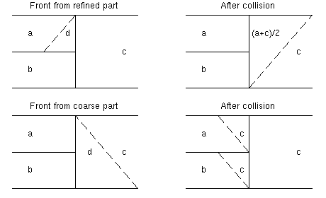
During the tracking phase, fronts may collide with the grid
interface. This is resolved by making the interface transparent, as
illustrated in Figure 4. Fronts coming from refined
tubes are collected, sorted according to wave speed, assigned new states as
illustrated in Figure 3, and inserted into the front
list in the coarse tube. Fronts coming in from a coarse tube are simply
inserted into each refined tube. Only in the special case of at least two
fronts colliding exactly at the interface do we solve a Riemann problem as in
Figure 3.

Figure 4: A single front colliding with a grid interface.
|
Adaptive Grid Refinement
The hyperbolic problems are time dependent, and therefore it is natural to
allow the refinement of the grid to vary with time also. Hence as the fine
structure move, so does the grid. By the nature of the algorithm, possible
refinements shold be determined in the projection step. One possible
criterion for determining refinement is the total variation inside each coarse
grid block. Before the projection, the solution consists of a set of
discontinuities with arbitrary spatial distribution. If the total variation
inside a coarse grid block exceeds an upper limit, the block is
refined. Similarly, if the total variation over all refined cells inside a
coarse block is below a lower limit, the block is made coarse again. Thus the
grid will be refined in regions with large total variation and coarse in
regions with small variation. By tuning the two threshold parameters, the
fraction of refined blocks varies.
The adaptive strategy improves the projection operator and provides better
initial data for the next step in the other direction. But we can still do
better. For instance, coarse blocks may be scattered in refined regions,
increasing the number of grid interfaces. In practise, a smoothing step is
included to preprocess the grid to reduce the number of interfaces.
Having determined the refined regions after one step, it is likely that the
structures will move during the next step. It would desireable if we were able
to determine this movement. This however, involves solving the Riemann problem,
which will be done in the front tracking step. Instead we can predict the
movement, by using an upper bound on the fastest wave emanating from the
refined section. This is possible to do for each specific flux function, but
is difficult to devise in general.
An stepwise demonstration of how the
algorithm works is available. See also movies of two computations of a Mach 3
wind tunnel with a step using small and large threshold parameters.
References
[1]
K.-A. Lie, V. Haugse, and K. Hvistendahl Karlsen:
Dimensional splitting with front tracking and adaptive grid
refinement.
Accepted in Numer. Methods Partial Differential Equations.
Knut-Andreas Lie <andreas@math.ntnu.no>
Last modified: Thu Jan 15 16:22:20 1998
