The finite element method#
Finite element methods are specific realizations of the Galerkin method. In a nutshell, the basis functions of the discrete function spaces are constructed from in three steps:
Generation of mesh \(\mcT_h = \{T\}\) which is a partition of the domain \(\Omega\) into smaller subunits \(T\), the mesh elements.
On each mesh element, a (local) finite dimensional function space \(V_T\) is constructed which has a fixed dimension.
The global discrete function space \(V_h\) is patched together suitably from the local, element-wise define function spaces. How the local function spaces are patched together will determine the resulting conformity of the global function space \(V_h\), e.g. whether \(V_h \subset L^2(\Omega)\) or \(V_h \subset H^1(\Omega)\). We start with the simplest 1D example to illustrate the most import concepts, before we formalize and extend those to cover the plethora of finite element families which exist out there today.
Finite element in 1D#
Consider a the finite interval \(\Omega = (a, b)\). To create a mesh, we introduce \(N+2\) nodes or vertices \(\{x_i\}_{i=0}^{N+1}\) such that \(a = x_0 < x_1 < \ldots < x_N < x_{N+1} = b\). Then the corresponding mesh \(\mcT_h = \{T_i\}_{i=1}^{N+1}\) is simply the finite collection of the \(N+1\) subelements \(T_i = [x_{i-1}, x_i]\) which are the mesh elements. We set mesh size \(h_T\)
As usual, for a set \(U \subset \RR^n\), we set \(\diam(U) := \sup \{\| \bfx - \bfy \| : \bfx, \bfy \in U \}\), which for our particular case means that \(\diam(T_i) = |x_i - x_{i-1}|\).
{.bg}
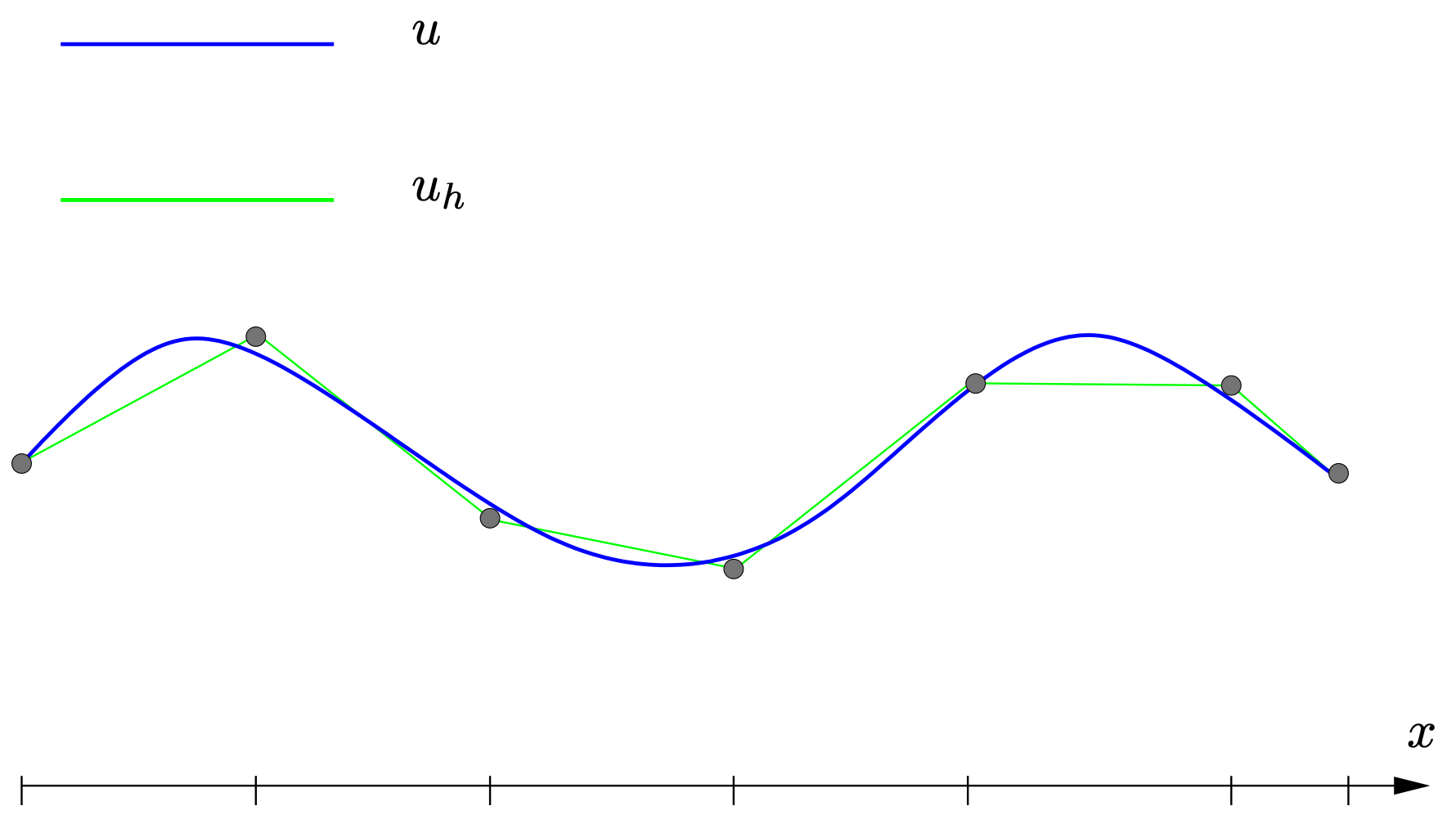
Continuous piecewise linear elements#
Next, we construct continuous, piecewise linear finite elements defined on \(\mcT_h\)
A typical function \(u_h \in \PPc_1(\mcT_h)\) approximating some function \(u\) is shown in the figure below.
TODO
Improve figure, denotes nodes and elements.
This global discrete function space can be constructed by defining suitably chosen basis functions for the space \(\PP_1(T_i)\) on each mesh element \(T_i\) and then patching them together to form a global basis for \(V_h\). Let’s focus on some element \( T = T_i = [x_{i-1}, x_i]\) for the moment and introduce the interpolation nodes \(\xi_0 = x_{i-1}\) and \(\xi_1 = x_i\), then our beloved Lagrange basis functions \(\{\phi_j^T\}_{j=1}^2\) are defined as the unique linear functions which satisfy
Here, we already note that the function evaluation \(\phi_j^T(\xi_k)\) can also be interpreted as evaluation of certain functionals \(\{\sigma_k \}_{k=0}^2\) if we define those functionals as follows
import ipywidgets as widgets
widgets.IntSlider(
    value=1,
    min=1,
    max=5,
    step=1,
    description='Element order:',
    disabled=False,
    continuous_update=False,
    orientation='horizontal',
    readout=True,
    readout_format='d'
)
If we repeat this construction on each element \(T_i\), we see that that elementwise defined basis functions are patched together to global, so-called hat functions \(\{\phi_i\}_{i=0}^{N+1}\) which satisfy \(\phi_j(x_i) = \delta_{ji}\) for a given mesh node \(x_i\) and which is linear on each element, see figure (TODO)
TODO
Add code with slider which shows the basis functions for different elements orders, both locally and the resulting functions in the global space.
Continuous piecewise quadratic elements#
We can repeat the entire procedure to construct piecewise quadratic elements. This time, we simply need to construct for each \(T \in \mcT_h\) the three Lagrange basis polynomials \(\{\phi^{T_i}_j\}_{j=0}^2\) which form a basis for the space \(\PP_2(T)\). Recall that after introducing the local interpolation nodes \(\xi_0 = x_{i-1}, \xi_{1} = x_{i-1} + h_i/2\), and \(\xi_{2} = x_{i}\), the local Lagrange basis polynomials are again characterized by the property
see figure (TODO). Again, the three functionals \(\{\sigma_k\}_{k=0}^2\) are defined as functionals which evaluates a given function in on of the respective interpolation points \(\xi_k\).
Repeating the construction on each \(T_i\) and patching those local basis functions together, we get elementwise quadratic functions of the following form:
TODO:
Add figure for P2
Next, we provide generalization with respect to the definition of meshes and the local finite elements.
Finite element method in several dimensions#
Meshes#
We start by giving a definition of a polyhedron (also called a polytope) which is taken and adapted from [Ern and Guermond, 2021] and which is suitable for our purposes.
Definition 6 (Polyhedron)
A polyhedron \(T\) in \(\RR^n\) is a compact interval if \(n=1\) and if \(n \geqslant 2\), it is compact, connected subset of \(\RR^n\) with non-empty interior such that its topological boundary \(\partial T\) can be written a finite union of images of affine mappings of polyhedra in \(\RR^{n-1}\).
A smooth polyhedron \(T\) is simply the image of a polyhedron by a smooth diffeomorphism.
Next, as we will mostly be concerned with simplical meshes, we need to recall the definition of a simplex as a particular instance of a polyhedron.
Definition 7 (\(d\)-simplex in \(\RR^n\))
A \(d\)-simplex \(S^d\) in \(\RR^n\) is defined as the convex hull of \(d+1\) vectors \(\{\bfa_0, \ldots, \bfa_d\} \subset \RR^n\), i.e.
The \(d\)-simplex \(S^d\) is call non-degenerated, if the vectors \(\bfb_i = \bfa_i - \bfa_0, i = 1,\ldots,d\) span a \(d\)-dimensional subspace of \(\RR^n\)
An \(l\)-dimensional face \(F = F(i_0, \ldots, i_l)\) of the \(d\)-simplex \(S^d(\bfa_0, \bfa_1, \ldots, \bfa_d)\) is defined as the convex hull
for a choice of indices \(\{i_0, \ldots, i_l\} \subset \{0, \ldots, d\}^{l+1}\). We also denote by \(\mcF^l(S^d)\) the collection of all \(l\)-dimensional faces of \(S^d\),
Usually, we call \(d-1\) dimensional faces for facets, \(0\)-dimensional faces for vertices and \(1\)-dimensional faces for edges.
A smooth non-degenerated \(d\)-simplex \(S^d\) is the image of a \(d\)-dimensional flat non-degenerated (reference) simplex \(\widehat{S}^d\) under a diffeomorphism \(\Phi : \widehat{S}^d \to S^d\). The \(l\)-faces of a smooth \(d\)-simplex are simply given by the image of the \(l\)-faces \(\widehat{F}\) under \(\Phi\).
Remark 5
With the definitions of the vectors \(\bfb_i\) above, note that we can rewrite the set of all convex combination as
With the definition of a —potentially smooth— polyhedron in place, we can introduce the concept of a mesh.
Definition 8 (Mesh)
A mesh \(\mcT_h = \{T\}\) for an open, bounded domain \(\Omega \subset \RR^n\) is a partition of \(\Omega\) into a collection of smooth polytopes \(T\), i.e.
TODO:
Add picture of more general polytopal meshes.
In this course, we will mostly use simplicial meshes, i.e. triangular meshes in \(\RR^2\) and tetrahedral meshes \(\RR^3\) which solely consist of respectively triangles and tetrahedrons. In such a case, every element \(T\) can be generated from a the (flat) simplex \(\widehat{T}\) (the reference element) via a geometric mapping \(\Phi_T : \widehat{T} \to T\) which we assume to be a smooth diffeomorphism. If the geometric mapping \(\Phi_T\) happens to be a affine mapping for all elements \(T\in\mcT_h\), the simplicial mesh is called affine.
For simplicial meshes, the references element is often chosen to be the unit simplex, i.e. the convex hull of the \(\mathbf{0} =: \bfe_0\) vector and standard orthonormal basis \(\{\bfe_1, \ldots, \bfe_n\}\):
From time to time, we might also consider quadrangular and hexahedral meshes where the elements are made up by smooth mappings of the standard unit-cube \([0,1]^n\). Again, we can introduce the concept of affine quadrangular meshes, but note that meshes can only consist of parallelograms and not general quadrangles.
Finally, we refine the concept of simplicial meshes more.
Definition 9 (Geometrically conform simplicial meshes)
A simplicial mesh \(\mcT_j = \{T\}\) is called geometrically conform if for any to simplices \(T, \widetilde{T} \in \mcT_h\), the intersection is an \(l\)-dimensional face of both \(T\) and \(\widetilde{T}\), for some \(0 \leqslant l \leqslant n\)