Advection-diffusion-reaction problems

In this chapter, we take a look at advection-diffusion-reaction (ADR) problems. We discuss briefly their well-posedness as well the occurrence of boundary layers which solution typically exhibits in the advection-dominated case, i.e. when the advection is much stronger than then diffusion. The section concludes with a short numerical example demonstrating the failure of a straight-forward and simple finite element discretization of an advection-dominant ADR problem.

Model problem

Let \(\Omega \subset \RR^d\) be an open and bounded domain. We try to find \(u: \Omega \to \RR\) such that

\begin{equation} \left\{ \begin{alignedat}{2} \mcA_{\epsilon} u = -\epsilon \Delta u + b\cdot\nabla u + c u &= f & &\quad \text{in } \Omega, \\ u &= g_D & &\quad \text{on } \Gamma = \partial\Omega, \end{alignedat} \right. \end{equation}

where

\begin{alignat}{2} & b: \Omega \to \RR^d &&\quad \text{ is the advection field}, \\ & c: \Omega \to \RR && \quad \text{ is the reaction term}, \\ & \epsilon > 0 && \quad\text{ is the diffusivity parameter.} \end{alignat}

Typical assumptions are

1. \(\epsilon \ll \|b\|_{\infty, \Omega}\) and \(\|c\|_{\infty, \Omega}\| \ll \|b\|_{\infty, \Omega}\) (advection-dominant)

2. \(\nabla\cdot b = 0 \) (flow field is incompressible) and \(c \geqslant 0\)

3. As an alternative to 2., one often requires that \( \inf_{x \in \Omega} (c(x) - \tfrac{1}{2} \nabla \cdot b(x)) \geqslant c_0 > 0\)

Later, we will need to distinguish between the inflow, outflow and characteristic parts of the boundary \(\Gamma\).

Definition 10 (Flow boundaries)

\begin{alignat}{3} &\text{Inflow boundary: } && \quad \Gamma^- = \{ x \in \Gamma: b(x) \cdot n(x) < 0 \} \\ &\text{Outflow boundary: } && \quad \Gamma^+ = \{ x \in \Gamma: b(x) \cdot n(x) > 0 \} \\ &\text{Characteristic boundary: } && \quad \Gamma^0 = \{ x \in \Gamma: b(x) \cdot n(x) = 0 \} \\ \end{alignat}

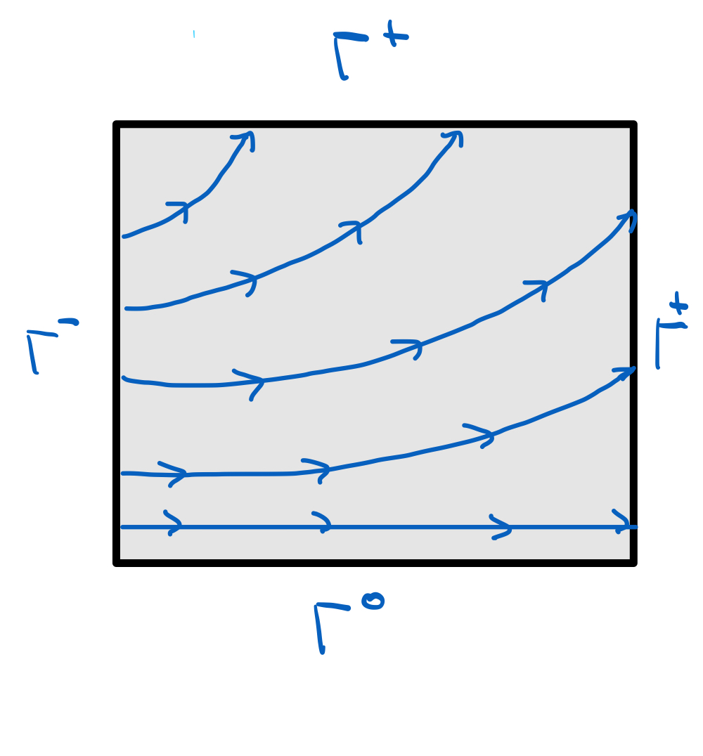
Fig. 2 The inflow, outflow and characteristic parts of the boundary \(\Gamma\).

For \(\epsilon \to 0\), we formally arrive at the reduced problem, which is of first order,

\[b\cdot\nabla u + cu = f \quad \text{in } \Omega \quad \text{supplemented with suitable b.c.}\]

But what are proper b.c. in the reduced case? Let us recall the method of characteristics.

Brief recap of the method of characteristics

The method of characteristics is a powerful tool to solve first order PDEs by transforming them into a system of ODEs, see e.g. [Evans, 2010], Chapter 3.2 or [Renardy and Rogers, 2004], Chapter 2 for a detailed introduction. In our particular case of the reduced problem, we need to determine the streamlines/characteristic curves \(\bfx(t, \bfx_0)\) of the flow field \(\boldsymbol{b}\) by solving

(45)\[\begin{split}\dfrac{d}{d\mrm{t}}\bfx(t, \bfx_0) &= \bfb(\bfx(t,\bfx_0)), \quad t > 0 \\ \bfx(0) &= \bfx_0.\end{split}\]

Note that thanks to well-known existence and uniqueness results for ODEs, if \(\bfb \in C^1(\Omega)\) the solution \(\bfx(t, \bfx_0)\) exists and that there is the map \((x_0, t_0) \mapsto \bfx(t, \bfx_0)\) is \(C^1\) and invertible. This allows us to establish a one-to-one correspondence between the solution of the ODE and the solution of the PDE.

Now the idea is to transform the PDE into a system of ODEs. First, we observe that If \(u\) solves the reduced problem (45), then \(\widetilde{u}(t, \bfx_0) := u(\bfx(t, \bfx_0))\) solves the ODE

\[\begin{split}\dfrac{d}{d\mrm{t}} \widetilde{u}(t; \bfx_0) &= \nabla u(\bfx(t, \bfx_0)) \bfb(\bfx(t, \bfx_0)) = f(\bfx(t, \bfx_0)) - c(\bfx(t, \bfx_0)) u(\bfx(t, \bfx_0)), \quad t > 0, \\ \widetilde{u}(t,\bfx_0) &= u_D(\bfx_0), \quad \bfx_0 \in \Gamma^-.\end{split}\]

In particular, we see that the solution \(\widetilde{u}\) incorporates the Dirichlet data \(u_D\) from the inflow boundary \(\Gamma^{-}\). Now we can solve the ODE for \(\widetilde{u}\) and then recover the solution \(u\) by setting

\[ u(\bfx) = \widetilde{u}(t, \bfx_0) \quad \text{where } \bfx = \bfx(t, \bfx_0). \]

It can then be shown that the \(u\) solves the reduced problem. Therefore, we conclude that for the reduced problem, we can only impose Dirichlet b.c. on the inflow part of the boundary, i.e. \(\Gamma^-\),

Definition 11 (Reduced problem for an advection-dominant ADR problem)

(46)\[\begin{split} b\cdot\nabla u + cu &= f_{\phantom{D}} \quad \text{in } \Omega, \\ u &= g_D \quad \text{on } \Gamma^-. \end{split}\]

For advection-dominant problems where \(\epsilon << 1\) the main challenge arise from the fact that on the one side, the solution \(u\) is expected to behave similiar to the solution of the reduced problem, and in particular, only requires Dirichlet b.c. on the inflow part of the boundary. On the other side, for \(\epsilon > 0\), the ADR problem is still elliptic and thus we need to impose Dirichlet b.c. everywhere and not only at the inflow boundary to render the problem well-posed, see also our discussion in the next Section Weak formulation and well-posedness of the advection-reaction-diffusion problem. As a results, we typically observe boundary layers in the solution \(u\) at the outflow boundary \(\Gamma^+\), where the solution \(u\) casually speaking rapidly transist from the solution of the reduced problem to the imposed Dirichlet boundary data, see Example 2: Trying to solve the previous example with a standard finite element method and Example 2: Trying to solve the previous example with a standard finite element method for an analytical and numerical example.