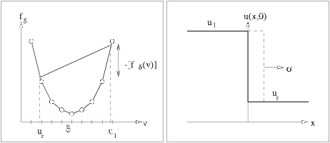
 Figure 1: Approximate solution of a Riemann problem giving a shock wave. |
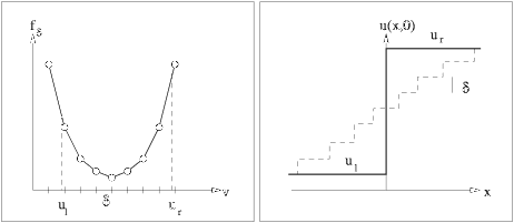 Figure 2: Approximate solution of a Riemann problem giving a rarefaction wave. |
Front tracking was first mentioned by Dafermos [2] in the 1970s. A related method had earlier been used by L.M. Barker [1] at Sandia National Laboratories in the late 1950s--early 1960s. Dafermos suggested the front tracking construction to study initial value problems for the scalar nonlinear hyperbolic equation. He observed that if the flux function is piecewise linear, the solution of the Riemann problem is within the class of step functions (piecewise constant). If the initial data is within this class, an analytical solution can be constructed by superposition of simple Riemann problems. The solution will remain piecewise constant for all time, since all wave interactions lead to new Riemann problems. By solving these Riemann problems a global solution can be established. In the general case, approximating the flux function by a sequence of piecewise linear functions and the initial data by a sequence of step functions gives a compact sequence of approximate solutions converging to the solution of the Cauchy problem.
Holden et al. [3] proved that Dafermos construction was well-defined, in that there is a finite number of steps in the algorithm, even for infinite time! They proposed to use the algorithm as an efficient numerical method. By changing the point of view slightly, Risebro [5] extended the front tracking method to systems of conservation laws. Instead of approximating the flux function, he suggested to approximate the solution of the Riemann problem to give solution within the class of step functions. This construction was used to give an alternative proof of existence of solutions for strictly hyperbolic systems of conservation laws. Risebro and Tveito [6,7] has later applied the method as an efficient computational tool for both the one-dimensional Euler equations as well as the nonstrictly hyperbolic polymer system in one-dimension
The front tracking method is closely related to the wave-front tracking algorithm used by Bressan and coworkers at SISSA.
See also the section on systems of hyperbolic equations.
We wish to study the problem
First, the flux function is approximated by a piecewise linear function and the initial data by a piecewise constant function. Then each Riemann problem in the initial data is solved.ut + f(u)x = 0, u(x,0) = u0(x).
A Riemann problem consists of two constant states
The solution is self-similar, u(x,t) = u(x/t) and is constructed as follows. If uL > uR we determine the upper concave envelope fc of the flux function f restricted to the interval [uR,uL], see Figure 1. If uL < uR we find the lower convex envelope fc, see Figure 2. Then the solution is determined from the equation y=fc'(u(y)), where y = x/t.u0(x) = uL, for x < 0
u0(x) = uR, for x > 0
 Figure 1: Approximate solution of a Riemann problem giving a shock wave. |
 Figure 2: Approximate solution of a Riemann problem giving a rarefaction wave. |
Figures 1 and 2 were drawn by Runar Holdahl
where each path of discontinuity is given by
u(x,t) = u1, for x < x1(t) u(x,t) = ui, for xi-1(t) < x < xi(t), i=2,...,N-1 u(x,t) = uN, for x > xN-1(t)
xi(t) = x0 + (t-t0)* [fc(ui+1) -fc(ui)]/ [ui+1-ui], or xi(t) = x0 + (t-t0)*si.
Then the solution of the (local) Riemann problems are connected to give the solution (global in x) up to the time of the first wave interaction. Before this time the solution can be determined by tracking the discontinuities (fronts). However, as pointed out above, a wave interaction is simply a new Riemann problem that can be solved as described above. Thus the global solution can be established by solving Riemann problems and tracking fronts.
The method can be extended to systems of hyperbolic conservation laws. Moreover, boundary conditions are easily included into the method.
The front tracking leads naturally to a very efficient numerical method. The method is grid independent in the sense that it needs no grid, except for specifying the piecewise constant initial data. The initial data can be specified on an arbitrary spaced grid and therefore represented very accurately. Moreover, convexity of the flux function is not important here. The method works for any non-convex flux function, as opposed to for instance methods based upon Roe-solvers, which typically need an entropy fix that can be quite elaborate to implement.
The most outstanding property of the method is that it is unconditionally stable, that is, there is no CFL condition restricting the possible time steps for a given spatial discretization. The time step is determined by the colliding fronts. Lucier [4] proved that the method is first order, even for discontinuous solutions.
Implementation of the method is discussed in a separate section.
The discretization parameters have been chosen very coarse with purpose in the examples below to clearly demonstrate the nature of the front tracking approximation.
Example 1. Burgers' equation with two Riemann problems in the initial data, (-1,0) and (0,1). The solution consists of two rarefaction waves, one from each Riemann problem, propagating in negative and positive direction, see Figure 3.
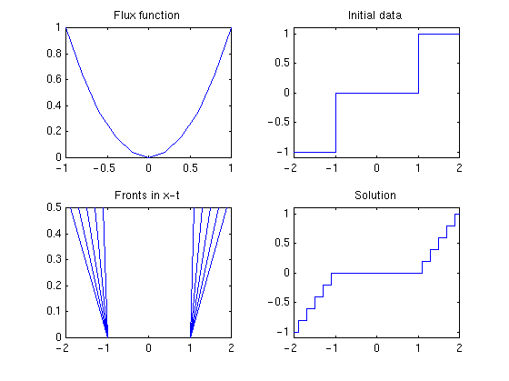 Figure 3: Example 1. |
Example 2. Burgers' equation with a two Riemann problems in the initial data, (1,0) and (0,-1). The solution consists of two shocks propagating towards the origin. As they meet, they form a single stationary shock (1,-1), see Figure 4.
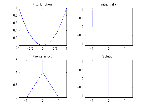 Figure 4: Example 2. |
Example 3. Consider a non-convex flux function f(u)=u3 and a truncated sinus function as initial data. The pattern of interacting fronts are slightly more complicated now, see Figure 5. However, since f'(u) is positive, all waves move in the positive direction.
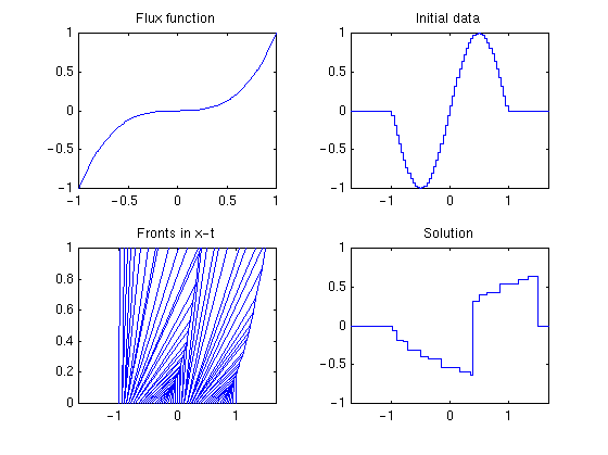 Figure 5: Example 3. |
Example 4. Finally, we consider a highly non-convex flux function f(u) = 2 u2(1-u2) with the same initial data as in Example 3. Since both the flux function and the initial data are symmetric, we get a symmetric wave pattern, see Figure 6. Now f'(u) changes sign, and accordingly we get waves moving i both directions.
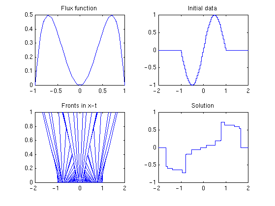 Figure 6: Example 4. |